to the abovementioned hypothesis about instrument errors,
we define three new errors: a cumulative angle error
d
γ
, an
attitude angle error
dμ
and a position error
dp
, which can be
expressed as:
=
=
=
=
,
,
= =
d d d d d d d dp dx dy
x
y
z
gc
gc
γ γ
γ
γ µ ω φ
=
(22)
Then, the horizontal error in x-axis and y-axis components
should have completely identical expression as:
dx dy
d d dp
f
f
= =
+
(
)
+
ρ γ
µ
2
2
2
2
.
(23)
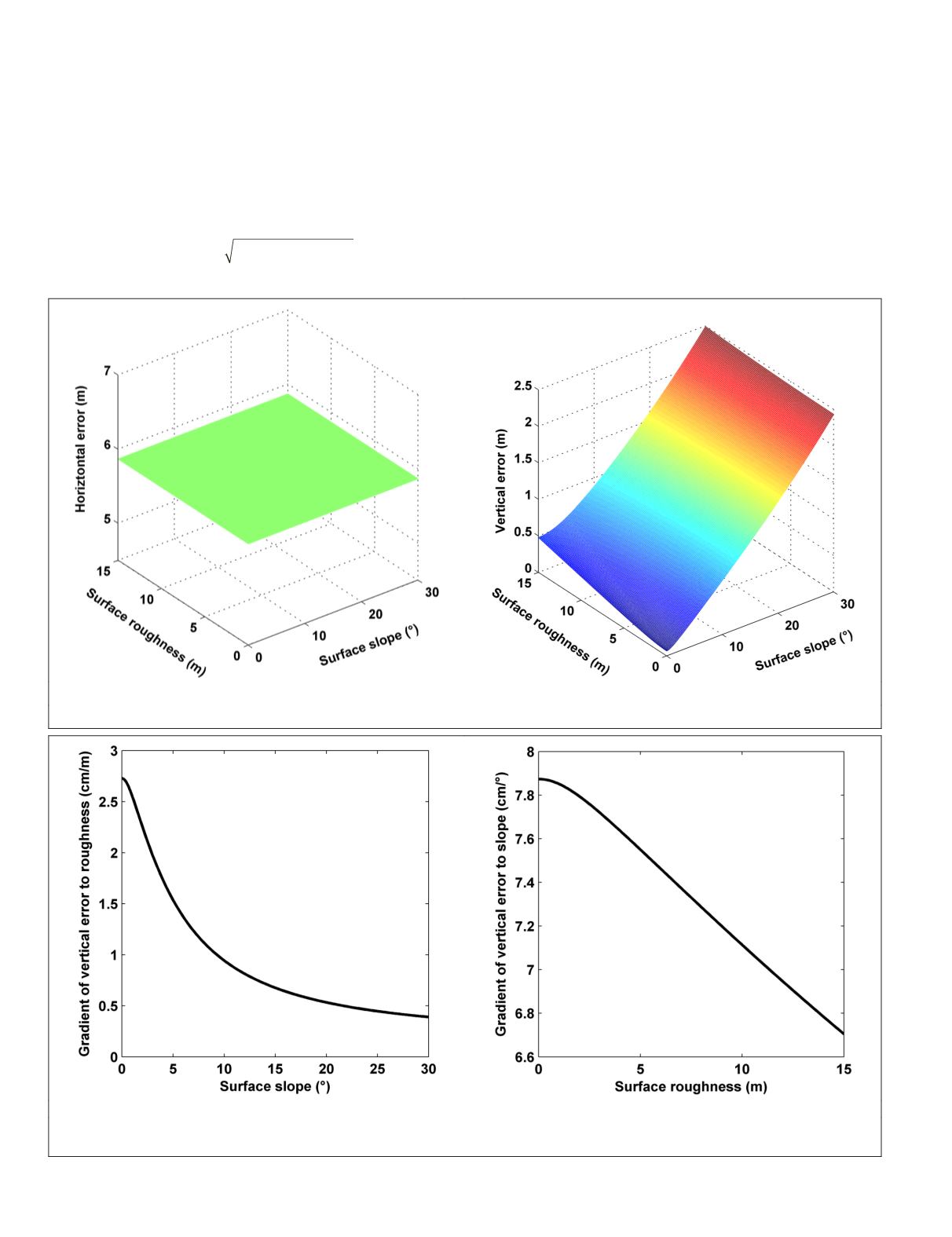
As shown in Figure 4a, the horizontal errors in x-axis
and y-axis components are constant and equal to 5.86 m.
However, the results from Figure 4) show that vertical error
raise rapidly from 0.07 m to 2.49 m with the increasing of
the surface slope and roughness. In other words, the vertical
errors in low-relief terrains cases are much less than those in
high-relief terrain cases. To evaluate the impact of the surface
slope and roughness on the vertical error, we calculate the
average gradient of the vertical error to the surface slope and
roughness,
g
r
and
g
s
, which can be found in Figure 5.
Figure 5a shows that the average gradient of the vertical
error to the surface roughness declines with the increasing of
the surface slope. When the surface slope is greater than 15
(a)
(b)
Figure 4. The
RMSE
of
LFG
distribution with the variability of surface slope and roughness: (a) horizontal error; and (b) vertical error.
(a)
(b)
Figure 5. The average gradient distribution of the vertical error to spatial parameters of terrain: (a) surface roughness; and (b)
surface slope.
652
October 2018
PHOTOGRAMMETRIC ENGINEERING & REMOTE SENSING


