resolution of the original
TI-HSI
dataset is 1.0 m, it can be seen
that such ambiguity can involve dozens of pixels at the 0.2-m
spatial resolution level.
Challenges Posed by the VIS Dataset
In addition to the well-studied problem of dealing with high
spatial resolution visible image classification, the large gaps
between the available strips aggravates the challenge.
For high spatial resolution imagery, the spatial information
can be of great assistance to the spectral information vari-
ability (Dalla Mura
et al.
, 2010; Huang and Zhang, 2011), and
can be extracted by a set of linear or nonlinear combinations
of the surrounding pixels. Although the spatial information
can improve the discriminability of the land-cover, it calls
for completeness in the spatial domain, and obvious spatial
structure corruption will decrease the performance of the
spatial descriptor. Unfortunately, due to the inconsistency of
the swath widths of the
VIS
and
TI-HSI
data, large image gaps
are found within the
VIS
data.
Proposed Method
The first important aspect for the classification is the dis-
criminative feature extraction. The following section analyzes
the spectral separability of the training sample set, as it can be
utilized as a foundation to improve the classification. The Jef-
fries-Matusita distance (JMD) and the transformed divergence
(
TD
) are two well-used evaluation indices for measuring the
degree of discriminability between two categories. The defini-
tions and physical meanings of these indices can be found in
Richards (1993). For the
VIS
dataset, it can be first observed
that the road/concrete class pair show weak separability, as
marked in bold in Table 2, and similar observations can be
made for the red roof/bare soil pair, due to the discriminative
limitation of the visible spectral information. For the
TI-HSI
dataset, the road pixels can be easily discriminated from the
rest of the classes, while the separability for the other class
pairs is poor.
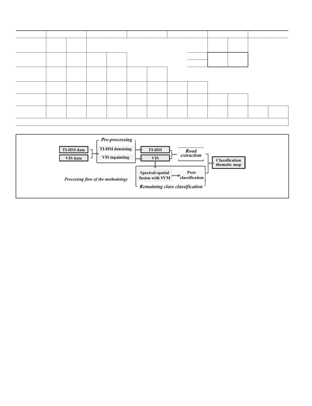
In view of the above phenomena, the entire classification
framework is composed of the following three parts: (a) data
pre-processing; (b) road extraction; and (c) remaining class
classification (see Figure 4).
Preprocessing
TI-HSI
Denoising and Dataset Matching
To alleviate the low-
SNR
problem, the first step of the pre-
processing procedure refers to noise removal with low rank
matrix recovery (Zhang et al., 2014). Considering the severe
noise, as shown in Figure 2c, the 82nd band is abandoned.
With regard to the different spatial resolutions of these two
datasets, calibration and resampling techniques are called for
in the matching step. The calibration procedure is based on
affine transformation. In fact, we just carry out the transla-
tion and isometric scaling without rotation, which is enough
for the following process. The reason for this is that the two
cameras are mounted on the same airborne platform, so the
LWIR
image and the
VIS
image are captured at almost the same
time and imaging conditions. In this way, upsampling by bi-
cubic interpolation of the denoised
TI-HSI
data is implemented
to match the
VIS
data at a finer spatial resolution. Bicubic
interpolation refers to cubic convolution interpolation, which
determines the gray level value from the weighted average of
the closest pixels to the specified input coordinates, and as-
signs that value to the output coordinates, in two dimensions.
In this way, the resulting image is slightly smoother than that
produced by bilinear interpolation, and it does not have the
staircase appearance produced by nearest neighbor interpola-
tion. It is suggested that there is less spectral distortion after
T
able
2. J
effries
-M
atusita
D
istance
and
T
ransformed
D
ivergence
for
the
VIS
and
TI-HSI D
atasets
Road
Trees
Red roof
Gray roof
Concrete roof
Vegetation
Trees
1.9975
1.9999
1.8556
1.9732
VIS TI-HSI
Red roof
1.8861
1.9992
1.8176
1.9102
1.9683
1.9997
0.8171
0.1635
JMD
TD
Gray roof
0.6343
0.7374
1.7233
1.8431
1.9447
1.9999
1.1751
1.3970
1.6400
1.9904
0.6226
1.0991
Concrete roof
1.7070
1.9259
1.6212
1.9408
2.0000
2.0000
1.0111
1.7344
1.9999
2.0000
0.6383
0.9885
1.8703
1.9999
0.9557
1.6675
Vegetation
1.9961
1.9999
1.8424
1.9219
0.9936
1.4547
0.4736
0.6372
1.9476
1.9841
0.9873
1.6496
1.9566
1.9999
1.2945
1.5322
2.0000
2.0000
1.0807
1.8971
Bare soil
1.9318
1.9600
1.9922
2.0000
1.9984
1.9998
1.9153
2.0000
1.3953
1.6779
1.9338
2.0000
1.9515
1.9615
1.9782
2.0000
1.9999
2.0000
1.8897
2.0000
1.9827
1.9964
1.8545
2.0000
Scope for both indices is [0,2] and >1.9
desirable separability, [1.4,1.8]
qualified sample, <1.4
bad classification result
Figure 4. Processing flow of the proposed method.
904
December 2015
PHOTOGRAMMETRIC ENGINEERING & REMOTE SENSING


