Then the error equation can be built as
v
s l
U X Y Z
U
x y i
x y i i
x y i i
i
first second third
,
,
, , ,
,
,
tan
,
, ,
=
(
)
(
)
+
(
)
ψ
z i i
i
X Y Z , ,
(
)
, (7)
where (
U
x
,
U
y
,
U
z
)
T
represents the right-hand part of Equation
6 and the calibration parameters are the corresponding ground
geodetic coordinates (
X
,
Y
,
Z
)
i
of the matched tie points and
the internal distortion parameters (
a
1
,…,
a
5
,
b
1
,…,
b
5
).
Internal-Parameter Estimation Method
In Equation 2,
a
0
represents the translation of the
LOS
along
the track and
b
0
represents the translation of the
LOS
across
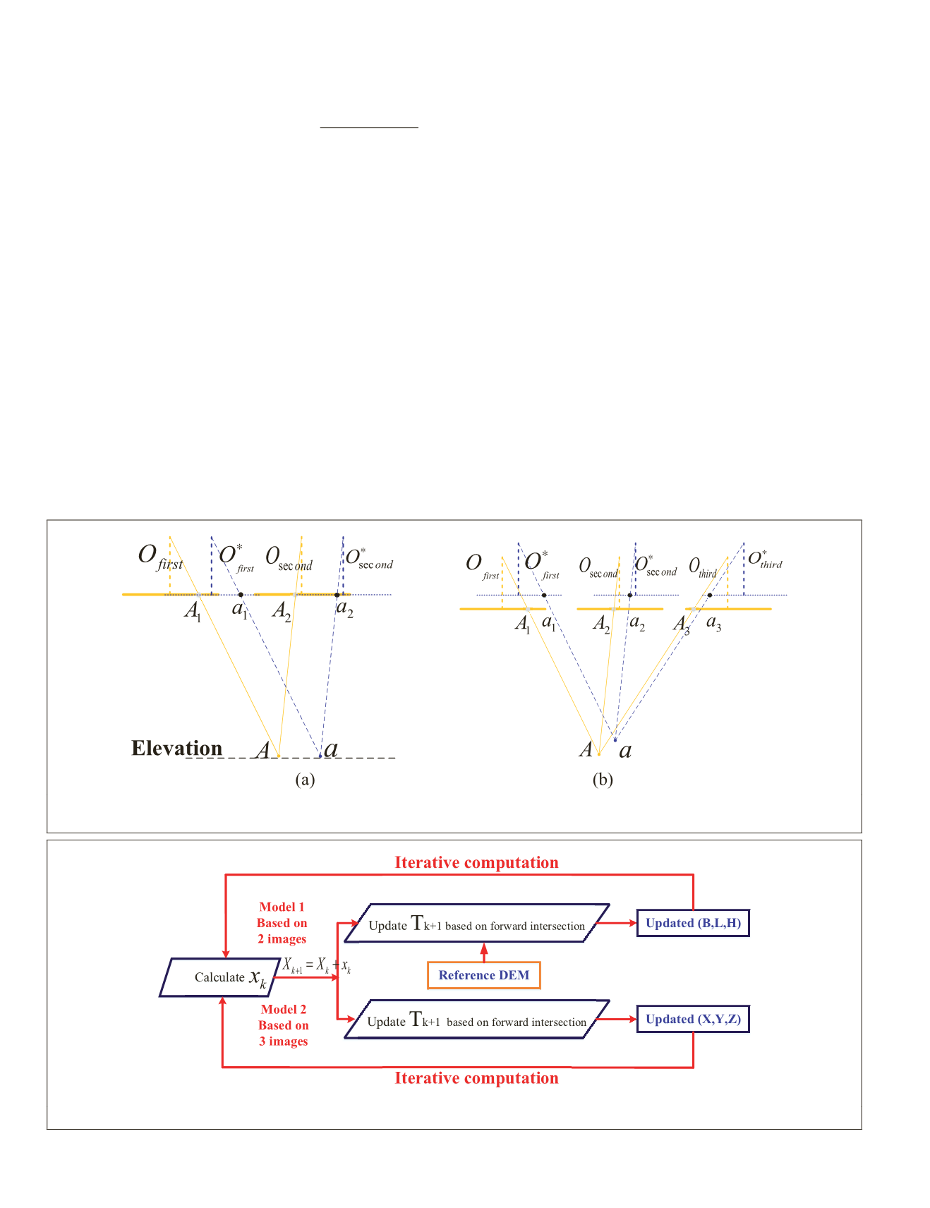
the track. As can be seen in Figure 8a, systematic translation
of the
LOS
would probably not bring the elevation residual
error, particularly under horizontal homogeneous geographi-
cal conditions. Similarly, systematic translation of the
LOS
would not bring the intersection residual error (Figure 8b).
Therefore,
a
0
and
b
0
are difficult to determine accurately by
the relative geometric constraint of the two self-calibration
models. The internal parameters of the primary
CCD
obtained,
based on a small-range calibration field, only compensate for
the distortion of the primary
CCD
;
a
0
and
b
0
could be reused
directly as the internal parameters
a
0
and
b
0
of the whole
CCD
for calibration (Wang
et al.
2014; Cheng
et al.
2018). Then the
internal parameters (
a
1
,…,
a
5
) and (
b
1
,…,
b
5
) can be calculated
based on the self-calibration models.
We can linearize Equations 5 and 7 in the
k
th iteration as
V
k
=
A
k
x
k
+
B
k
t
k
–
L
k
,
(8)
where
X
k
= (
a
1
,…,
a
5
;
b
1
,…,
b
5
)
k
T
and
x
k
=
Δ
X
k
correct the internal
distortion parameters:
T
k
= (
B
1
,
L
1
,
B
2
,
L
2
,…,…,
B
N
tie
,
L
N
tie
,)
k
T
in
Equation 5 for paired stereoscopic images, and
T
k
= (
X
1
,
Y
1
,
Z
1
,
X
2
,
Y
2
,
Z
2
,…,…,
X
N
tie
,
Y
N
tie
,
Z
N
tie
)
k
T
in Equation 7 for three ste-
reoscopic images.
N
tie is the number of matched tie points;
t
k
=
Δ
T
k
is the correction vector of the object point coordinates;
and
V
k
is the residual error vector. The design matrices
A
k
and
B
k
contain the partial derivatives of the calibration parameters
calculated by image-space and object-space measurements.
The
LOS
difference vector in image space of the tie points
L
k
can be calculated by the current internal parameters, and we
use
P
k
to represent the weighted matrix of the tie points.
Using a least-squares estimation, we can build
A P A A P B
B P A B P B
x
t
A P L
B P
k k k k k k
k k k k k k
k
k
k k k
k
T
T
T
T
T
T
=
k k
L
.
(9)
As shown in Figure 9, to simplify the calculation the in-
ternal calibration parameters
x
k
were calculated first, and
T
k
+1
can be updated based on the forward intersection. The itera-
tive computation was needed in the calculation flow.
Figure 8. Systematic translation of the charge-coupled device detector. (a) Influence of the systematic translation for paired
stereoscopic images; (b) influence of the systematic translation for three stereoscopic images.
Figure 9. The calculation flow of the internal calibration parameters.
820
November 2019
PHOTOGRAMMETRIC ENGINEERING & REMOTE SENSING


