Algorithm 1. Optimized Endmember Extraction
Based on K-SVD
Input:
Hyperspectral data matrix
X
∈
R
L
×
N
.
Output:
Estimated endmembers ˆ
A
= [ ˆ
a
1
, ˆ
a
2
, …, ˆ
a
P
,].
Initiation:
A
0
(Obtain by the classical method).
S
0
(Obtain by the fully constrained least squares).
X
,
A
0
each column is normalized to a unit
l
2
-norm.
Step 1. Preprocessing
:
Get an appropriate threshold of
S
;
Select the data
X
within the threshold for the next calculation.
Step 2. Eliminate background noise
(
J
= 0)
Define the residual matrix
R
δ
by Equation 11.
Calculate the mean of the residuals for each band –
r
i
δ
by
Equation 12.
Obtain the image matrix after removing background noise
~
X
by Equation 13.
Step 3. Iteratively updating endmembers:
For each column
p
= 1,2, …,
P
;
Define
ω
p
= {
j
|1
≤
j
≤
N
,
S
T
P
(
i
)
≠
0} to record the nonzero posi-
tion in
S
T
P
.
Calculate the
p
th
endmember residual matrix
E
P
by Equation 10.
The error matrix
E
p
is constrained according to the matrix
ω
p
,
E
R
p
=
E
p
×
ω
p
.
Apply
SVD
:
SVD
(
E
R
p
)=
U
Δ
V
T
. Update endmember vector by ˆ
a
P
=
U
(:,1) and corresponding coefficient vector by
S
T
P
=
Δ
(1,1) ×
V
(:,1).
Stop condition:
The update of | ˆ
A
[
J
]
– ˆ
A
[
J
– 1]
| is small enough, otherwise
J = J
+ 1 and repeat.
Experiments and Analysis
The spectral angle distance (
SAD
) is used to evaluate the end-
member accuracy, which is a high-dimensional extension to
the two-dimensional geometric angle defined as follows:
SAD
P
p
T
P
P
=
−
cos
1
a a
a a
where,
a
p
and ˆ
a
P
denote the standard endmember signa-
ture and estimated endmember signature, respectively. The
symbol
|
·
|
represents the Frobenius norm. The
SAD
value is
smaller; the estimated endmember is closer to the standard
endmember. D-value is described as Equation 15.
D-value SAD
before
mean
KSVD
mean
SAD
=
−
(15)
where,
SAD
is the mean value of
SAD
obtained from the
method before optimized,
SAD
is the mean value of
SAD
obtained from the method after optimized. D-value is used to
evaluate the degree of optimization. The D-value is larger; the
degree of the optimization is higher.
overall
D-value
SAD
before
mean
=
(16)
The overall value is calculated by the ratio between the
D-value and the
SAD
. The overall value indicates the
accuracy increase rate after the optimization, calculated as
Equation 16.
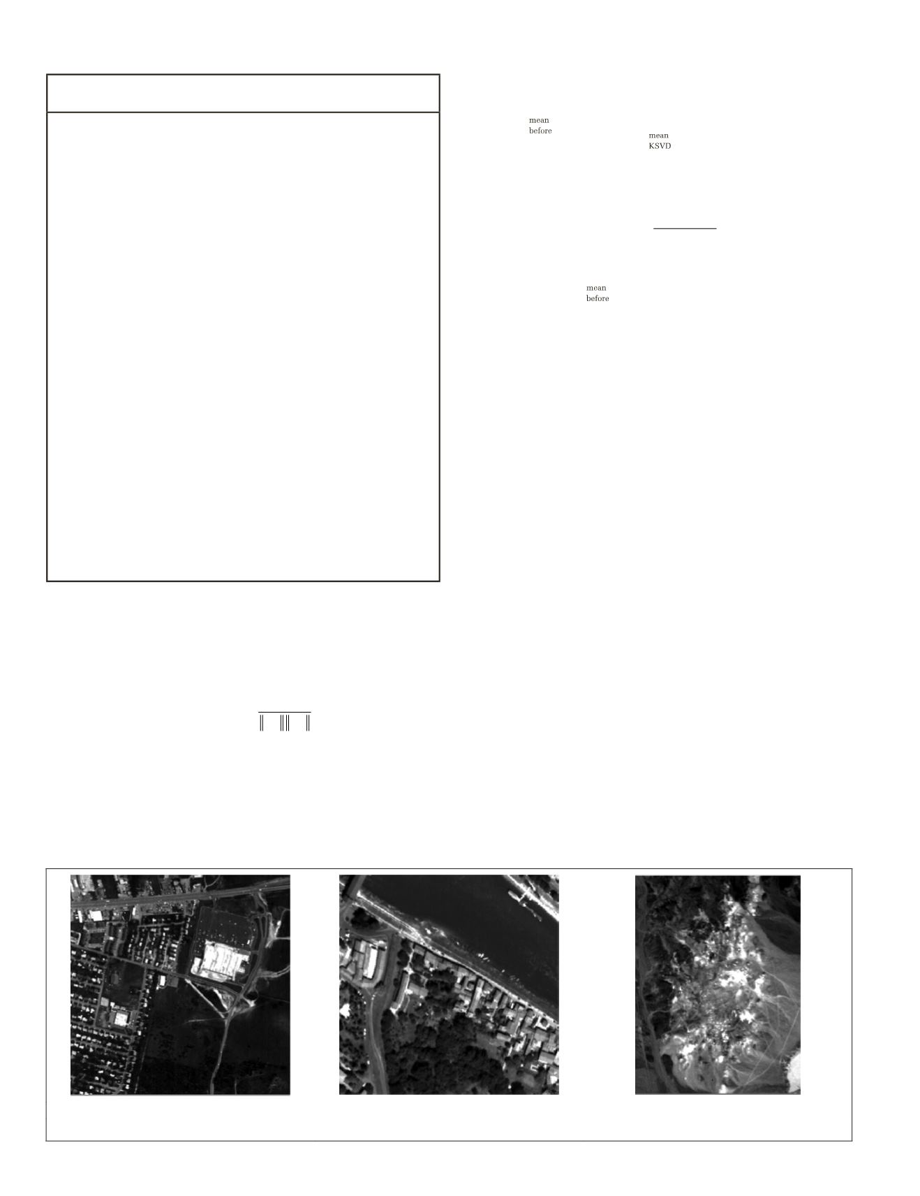
Experiment Data set
The first
HSI
dataset was captured by the Hyperspectral Digital
Imagery Collection Experiment (
HYDICE
) over the urban in
Copperas Cove, the data was obtained from the U.S. Army
Center
/
FactSheetArticleView/tabid/9254/Article/610433/hypercube.
aspx). The image includes 210 bands, which cover the wave-
length of 400 to 2400 nm, and spectral resolution is 10 nm.
After the removal of low-
SNR
and water absorption bands (1–4,
76, 87, 101–111, 136–153, and 198–210), 162 bands remain.
The image size is 307×307 pixels, shown in Figure 1a. There
are six classes in this dataset: asphalt road, concrete road,
grassland, roof, roof shadow, and tree. The corresponding ref-
erence spectral signatures are chosen from the spectral library
available online at
.
The second dataset was captured by the Reflective Optics
System Imaging Spectrometer 03 (ROSIS) over Pavia city,
which was provided by the Data Fusion Technical Commit-
tee. There are 115 bands of the image, but some channels are
removed due to the noise, so the image includes 102 bands
that cover the wavelength of 430 to 860 nm. The spatial reso-
lution of the image is 1.3 m. The size of selected subscene is
250×250 pixels shown in Figure 1b with the residential area
on the side of the river Ticino. There are six classes in this
ad, roof, tree, and water.
as the subimage of the Cuprite data
Visible/Infrared Imaging Spectrometer
(
AVIRIS
) in June 1997 in Nevada, USA. The dataset was down-
loaded from the United States Geological Survey website
(
) and the
dataset included 224 bands covering the wavelength range of
370 to 2480 nm. After removing the low
SNR
bands (1–3 and
221–224) and water absorption bands (106–115 and 151–169),
(a) Urban
(b) Pavia
(c) Cuprite
Figure 1. The image of the (a)
HYDICE
Urban, (b)
ROSIS
Pavia, and (c)
AVIRIS
Cuprite dataset.
882
December 2019
PHOTOGRAMMETRIC ENGINEERING & REMOTE SENSING


