Table 5 reports the processing times for four optimized
methods (unit of time is in seconds). All the algorithms are
implemented using
MATLAB
R2018a on a desktop computer
equipped with an Intel quad-core central processing unit (at
3.7
GHz
) and 16 GB of
RAM
memory. From Table 5 it can be
seen that the size of imagery is the main factor affecting the
speed of the process. While the iteration process, the column
vector of the endmember matrix remains normalized, so the
optimization is fast.
Conclusion
This paper proposes an optimization endmember extraction
method based on
K-SVD
. Our contribution includes three parts.
(1) The proposed method reduces the calculations by select-
ing the
HSI
data based on an appropriate threshold, which
is obtained by the abundance value. In order to ensure the
correctness of the selected threshold, we provide detailed
SAD
and D-value changing curves. (2) The use of the gross error
elimination removes the average residual of each band from
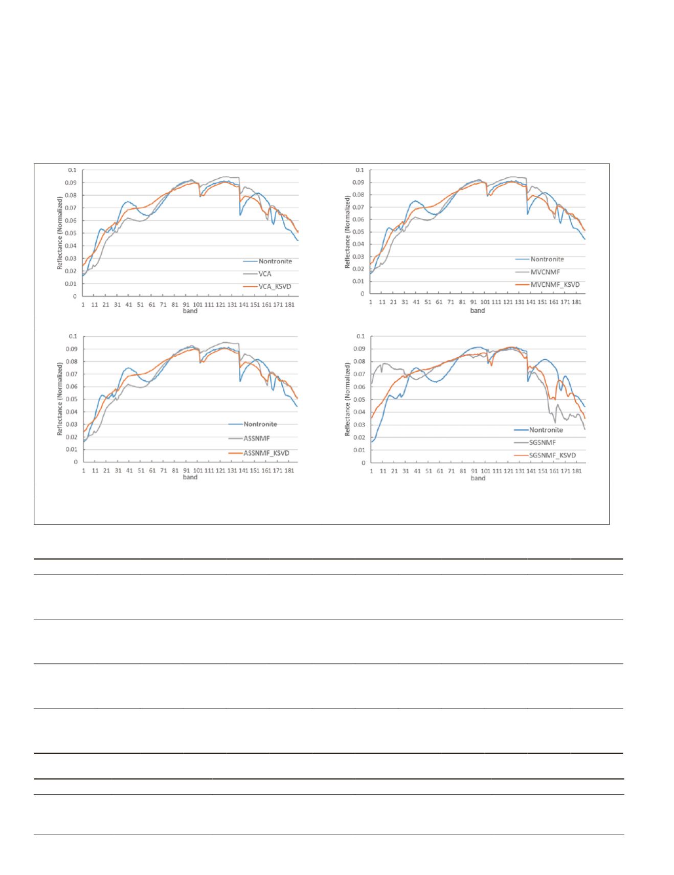
(a) VCA_KSVD
(b) MVCNMF_KSVD
(c) ASSNMF_KSVD
(d) SGSNMF_KSVD
Figure 5. Comparison of the extracted Nontronite using the optimized methods with the standard curves in Cuprite
dataset.
Table 4. SADs between reference spectr
before and after optimized on Cuprite
dataset.
Endmembers
1
2
3
4
5
6
7
8
9
10
Mean Overall, %
VCA
before
0.1889 0.0978
0.1612
0.0751
0.1862
0.1012
0.1041
0.1069
0.0714
0.0983
0.1191
15.3
after
0.1962 0.0707
0.1280
0.0661
0.1601
0.0704
0.0718
0.0749
0.0745
0.0961
0.1009
D-value
-0.0073 0.0271
0.0332
0.0090
0.0262
0.0308
0.0324
0.0321 -0.0031
0.0022
0.0183
MVCNMF
before
0.0629 0.1908
0.1203
0.0615
0.0880
0.0798
0.1055
0.1272
0.1123
0.0788
0.1027
17.7
after
0.1978
0.0692
0.1280
0.0661
0.1554
0.0728
0.0735
0.0751
0.0740
0.0963
0.1008
D-value
-0.0088
0.0282
0.0323
0.0095
0.0307
0.0286
0.0307
0.0317 -0.0031
0.0023
0.0182
ASSNMF
before
0.1899
0.0971
0.1620
0.0697
0.1858
0.1015
0.1080
0.1074
0.0638
0.1108
0.1196
15.8
after
0.1978
0.0693
0.1272
0.0663
0.1590
0.0692
0.0723
0.0751
0.0737
0.0970
0.1007
D-value
-0.0080
0.0278
0.0348
0.0034
0.0268
0.0322
0.0357
0.0323 -0.0100
0.0138
0.0189
SGSNMF
before
0.1012
0.1268
0.1116
0.0792
0.1759
0.0808
0.1105
0.1759
0.0462
0.1487
0.1157
15.1
after
0.0796
0.1122
0.1239
0.0653
0.1455
0.0781
0.0806
0.1375
0.0560
0.1036
0.0982
D-value
0.0216
0.0146
-
0.0123 0.0140
0.0304
0.0027
0.0299
0.0384
-
0.0098 0.0451
0.0175
Table 5. Time comparison of three datasets for different optimized methods (unit: seconds).
Dataset (pixels)
VCA_KSVD
MVCNMF_KSVD
ASSNMF_KSVD
SGSNMF_KSVD
Urban (307×307)
408.754
441.959
174.825
904.347
Pavia (250×250)
716.190
117.893
123.913
129.579
Cuprite (250×190)
98.739
127.225
47.875
131.910
886
December 2019
PHOTOGRAMMETRIC ENGINEERING & REMOTE SENSING


