the image includes 188 bands and the size is 250×190 pixels,
shown in Figure 1c. According to the ground truth of differ-
ent mineral materials in the image, 10 kinds of endmembers
were selected for endmember extraction in this experiment:
Alunite, Andradite, Buddingtonite, Dumortierite, Kaolinite1,
Kaolinite2, Muscovite, Nontronite, Pyrope, and Chalcedony.
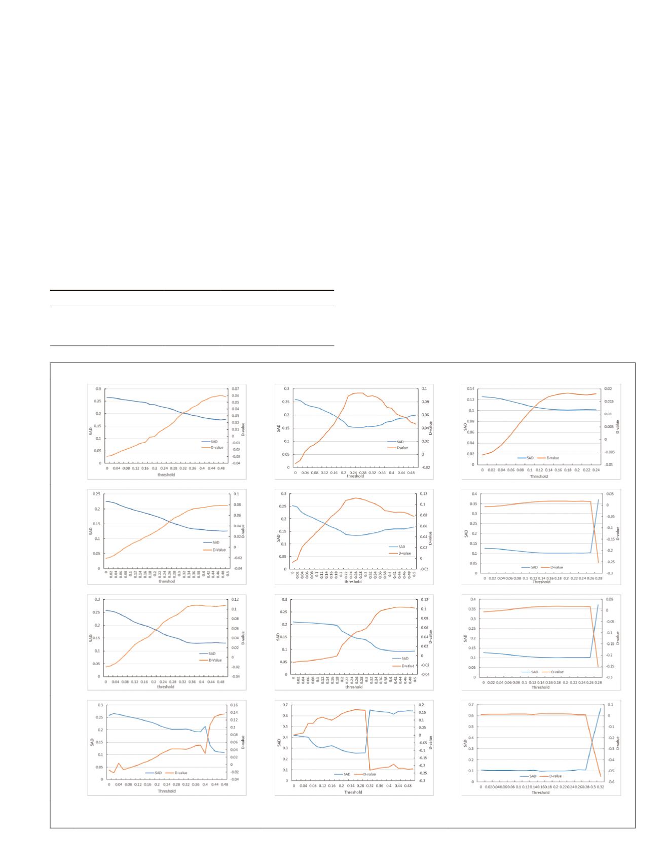
Threshold Value Change Analysis
This section will discuss the way to select the appropriate
threshold through the
SAD
and D-value variation curves (see
Figure 2).
As the
SAD
curve reaches the minimum and the D-value
curve reaches the maximum, the corresponding threshold
value is chosen. We choose the extreme value of the curve;
the lowest point of the
SAD
curve is also the highest point of
the D-value curve. Every dataset has its own threshold, which
is shown in Table 1.
Experiment Results
Figure 3 clearly shows that the
K-SVD
optimized methods’
results are superior to the original methods. The reference
curve and curve from the proposed method are very close,
especially in Figures 3c and 3d. The details of the curves are
also restored better than the original methods.
Table 2 shows the endmember extraction accuracy of the
HYDICE
urban dataset. Shadow in Table 2 means roof shadow.
Except for tree, all five species have been optimized to dif-
ferent degrees. According to the D-value, after the optimiza-
tion,
MVCNMF
obtained the best results of the Asphalt, Grass
and Roof, and the D-value is 0.0822, 0.0199,0.0906;
SGSNMF
obtained Concrete and Shadow in the best results, and the
D-value 0.0535 and 0.2339. After optimization, the D-value of
Concrete obtained by
VCA
is 0.1064; the D-value of Shadow
obtained by
MVCNMF
is 0.2893; D-value of Shadow obtained
by
ASSNMF
is 0.3252; D-values of Shadow and Asphalt
obtained by
SGSNMF
are both about 0.23. The results from
SGSNMF
has the most obvious optimization, especially in
Asphalt and Shadow.
For the
VCA
algorithm, the mean
SAD
decreases from 0.2359
to 0.1754 and the overall optimization reaches 25.6%. For
the
MVCNMF
algorithm, the mean
SAD
decreases from 0.2052
to 0.1260 and the overall optimization degree reaches 38.6%.
For the
ASSNMF
algorithm, the mean
SAD
decreases from
0.2381 to 0.1300 and the overall optimization degree reaches
45.4%. For the
SGSNMF
algorithm, the mean
SAD
decreases
Urban
Pavia
Cuprite
(a)
(b)
(c)
(d)
Figure 2. The
SAD
curve and
D
-value curve change with the increase of threshold. (a)
VCA_KSVD
, (b)
MVCNMF_KSVD
, (c)
ASSNMF_
KSVD
, and (d)
SGSNMF_KSVD
for endmember extraction from Urban, Pavia, and Cuprite datasets, respectively.
Table 1. Different thresholds for three datasets.
Dataset
VCA MVCNMF ASSNMF SGSNMF
Urban
0.48
0.48
0.38
0.48
Pavia
0.28
0.26
0.44
0.26
Cuprite
0.18
0.18
0.18
0.16
PHOTOGRAMMETRIC ENGINEERING & REMOTE SENSING
December 2019
883


